How to Freeze Rows and Columns in Excel

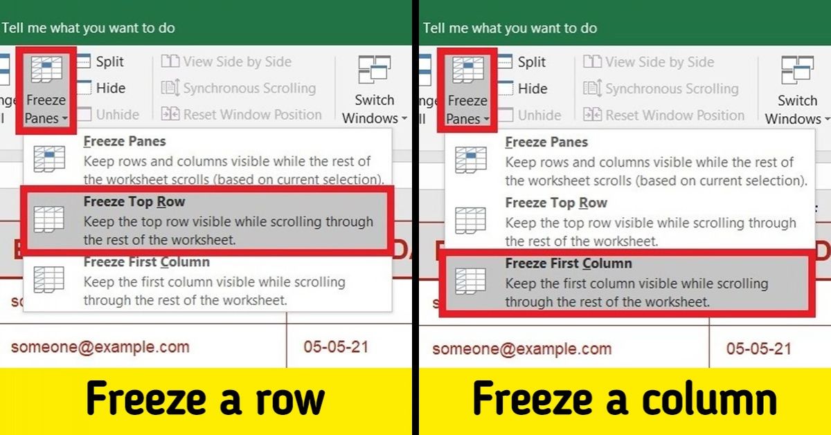
If your Excel spreadsheet contains a lot of data, it can be difficult to work with. After all, it is one thing to compare information on several rows, and another — when there are several dozen of them. In these cases, freezing areas with the important data, that you use most often, can help.

5-Minute Crafts prepared a guide for you on how to freeze or unfreeze rows and columns in Excel.

1. Freeze the top row

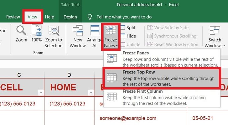
On the View tab, in the Window group, click Freeze Panes. Then click Freeze Top Row. Now scroll down to the rest of the worksheet. Excel automatically adds a dark grey horizontal line to indicate that the top row is frozen.

2. Freeze the first column

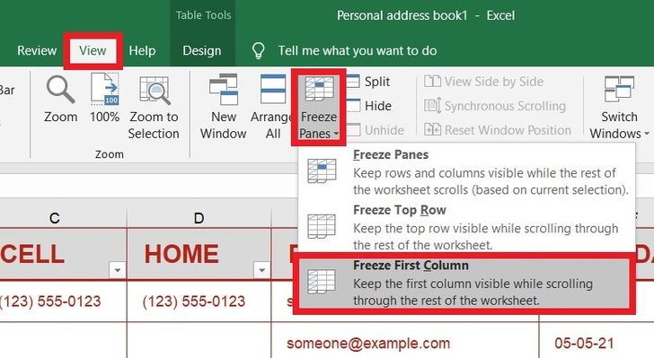
On the View tab, in the Window group, click Freeze Panes. Then click Freeze First Column. Now scroll to the right of the worksheet. Excel automatically adds a dark grey vertical line to indicate that the first column is frozen.

3. Freeze the top row and the first column

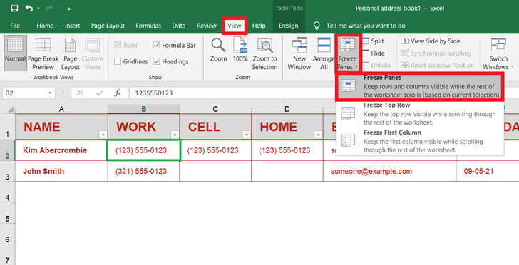
Select the cell below the top row and to the right of the first column that you want to keep visible when you scroll. On the View tab, click Freeze Panes, and then choose Freeze Panes. After that, the top row and the first column will be frozen during scrolling.

4. Unfreeze rows and columns

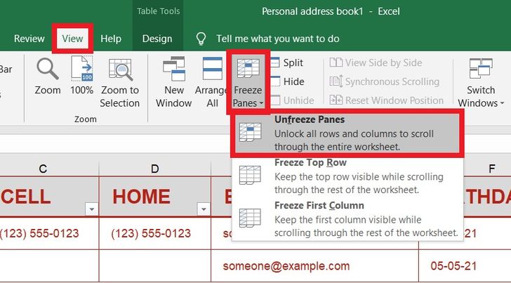
On the View tab, click Freeze Panes, and then choose Unfreeze Panes. After that all rows and/or columns will be unlocked and may not be visible when you scroll down your worksheet.